
|
|
| . |
Scaling PID Tuning Parameters for Different Controller Sample RatesIntroductionWhen tuning servo systems, it may be necessary to adjust the controller's sample rate for optimum performance. Changing the sample rate will directly affect the closed loop response of the PID control algorithm. To maintain stability and performance, the PID parameters must be scaled to match the change in sample rate. This document explains how to scale the tuning parameters properly. This document only addresses scaling for the PID closed loop algorithm. It does not compensate for resonances caused by increased system bandwidth or system nonlinearities.
WARNING! The system may experience stability problems when sample rates are changed from a higher sample rate to a much lower sample rate. This is due to additional phase lag of the zoh (zero order hold, the value that is held constant between sample periods) at a lower sample rate. It is necessary to take the appropriate safety precautions in order to prevent any sudden and unexpected movement of machinery from being hazardous to neighboring objects and/or personnel. Before entering or changing sample rates, verify that all personnel, hands, fingers, body parts, and/or property are clear of the movement area; otherwise, injury or death may result! PID Loop and Sample RatesWhen sample rates are changed, the performance of the servos will change. To understand why this relationship exists, it is helpful to look at the architecture of a PID control loop. PID Feedback LoopsA simplified PID feedback loop is shown in the diagram below.
Major Components of the PID Feedback Loop,
|
||||||||||||||||||||||
|
Kp does not need to be compensated for when using different sample rates because the proportional term has no time component.
The equation that the XMP uses for the integral term
provides insight into how to compensate for the change in sample rate.
If you look at the difference between the XMP integral term and the ideal
digital derivative term, you will find that the XMP derivative term should
be multiplied by the sample (tsample) to change it to the ideal
digital derivative term. This means that you only need to multiply by
the sample period (tsample) or divide by the sample rate (1/
tsample) to compensate for a sample rate change.
![]()
![]()
Example - Ki
Integral Term
To convert Ki from one sample rate to another, multiply by the new sample
rate and divide by the old sample rate.
old Ki = 0.01
old SR = 2,000
new SR = 10,000
new Ki = old Ki * (old SR / new
SR) = 0.01 * 2,000 / 10,000 = 0.002
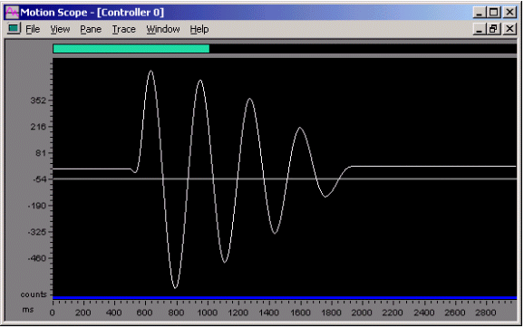
Figure 2. External Disturbance Kp = 10, Ki = 0.01, SR = 20,000
The graph above shows a system that is almost in a state of instability due to a large integral term and a lack of a derivative term. Actual position is plotted vs. time showing an external disturbance.

Figure 3. External Disturbance Kp = 10, Ki = 0.01, SR = 10,000
The integral term (Ki) is effectively larger at a 10,000Hz sampling rate than a 2,000Hz sampling rate. This increase in integral gain results in an unstable case, as shown in the diverging oscillation in Figure 3.
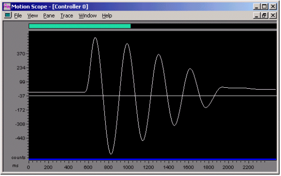
Figure 4. External Disturbance Kp = 10, Ki = 0.002, SR = 10,000
When the integral term is properly compensated for by using a smaller compensated integral term, it will result in performance that is very similar to the original performance. Notice the similarity between the graphs of Figure 2 and Figure 4.
The equation that the XMP uses for the derivative term provides insight into how to compensate for the sample rate change.
If you look at the difference between the XMP derivative term and the ideal digital derivative term, you find that the XMP derivative term should be divided by the sample (tsample) to change it to the ideal digital derivative term. This means that you only need to divide by the sample period (tsample) or multiply by the sample rate (1/ tsample) to compensate for a sample rate change.
![]()
![]()
Example
To convert Kd from one sample rate to another, multiply the old Kd by
the new sample rate and divide by the old sample rate.
old Kd = 1,000
old SR = 2,000
new SR = 10,000 (Kd * new SR) /
old SR = (1,000 * 10,000) / 2,000 = 5,000
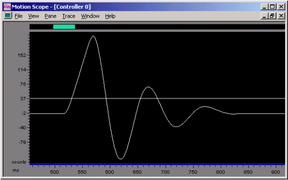
Figure 5. External Disturbance
Kp = 100, Ki = 0, Kd = 1,000, SR = 2,000
The graph above shows actual position vs. time where the system is subjected to an external disturbance. The system is tuned to be somewhat underdamped.
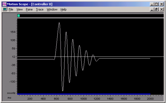
Figure 6. External Disturbance
Kp = 100, Ki = 0, Kd = 1,000, SR = 10,000
Notice that the system has less dampening at a higher sample rate with the same tuning parameters. Next, we will compensate the derivative term for the change in sample rate.
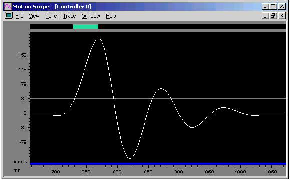
Figure 7. External Disturbance
Kp = 100, Ki = 0, Kd = 5,000, SR = 10,000
Notice that the disturbance plots at 2,000Hz and 10,000Hz are nearly identical when the PID parameters are compensated for the sample rate.
A simplified diagram of the PID feedforward loop is shown below.
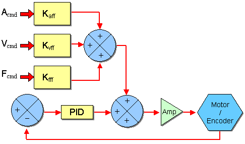
Figure 8.
|
Kaff is calculated as the command acceleration counts / controller sample2 multiplied by Kaff. In order to compensate for acceleration feedforward, convert from (counts / controller sample2) to (counts / second 2) for the original sample rate and back using the new sample rate.
new Kaff = (new SR / old SR)2 * old Kaff
Example
Let's say you have a sample rate of 2,000 Hz with a Kaff value of 100,000.
To convert the original sample rate from (counts / controller sample2)
to (counts / second2) and back using the new sample
rate, multiply Kaff by the square of the new (SR / old SR).
old SR = 2,000
new SR = 10,000
old Kaff = 100,000
new Kaff = (new SR / old SR)2
* old Kaff = (10,000 / 2,000)2 * 100,000 = 2,500,000
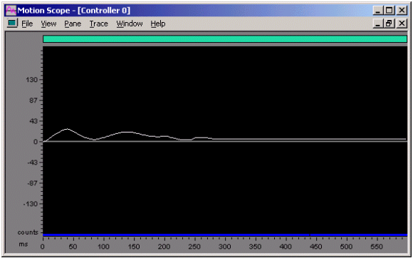
Figure 9. External Disturbance
Kp = 100, Ki = 0, Kd = 5,000, SR = 10,000
The above graph shows position error vs. time for a commanded motion with an underdamped servo system. The underdamped nature of the system is difficult to see because the loads on the system are largely inertial. The acceleration feedforward nearly eliminates any inertial based position error.

Figure 10. Position Error for a Commanded Motion
Kaff = 100,000, SR = 10,000
PID parameters scaled from values used at SR = 2,000
This stage was intentionally tuned to be underdamped, highlighting an incorrect acceleration feedforward. Notice that large position errors occured because the acceleration feedforward value was not scaled with the change in sample rate (SR).

Figure 11. Position Error for a Commanded Motion Kaff = 2,500,000, SR
= 10,000 PID parameters and Kvff scaled for changed sample rate
Notice that when Kaff is changed, the position error is greatly reduced and a profile is produced that is very similar to the graph made at SR = 2,000. See Figure 9 and Figure10.
Kvff is calculated as the command velocity counts / controller sample multiplied by Kvff. In order to compensate for velocity feedforward, convert from (counts / controller sample) to (counts / second) for the original sample rate and back using the new sample rate.
new Kvff = (new SR / old SR) * old Kvff
Example
Let's say you have a sample rate of 2,000 Hz with a Kvff value of 100,000.
To convert from (counts / controller sample) to (counts / second)
for the original sample rate and back using the new sample rate, multiply
Kvff by the ratio of the new to old sample rate (SR / old SR).
old SR = 2,000
new SR = 10,000
old Kvff = 100,000
new Kvff = (new SR / old SR) * old Kvff
= (10,000 / 2,000) * 45 = 225

Figure 12. Position Error vs. Time for a Commanded Motion
Kvff = 45, SR = 2,000
Here is the same move on the same stage as used for the acceleration feedforward example was performed, except velocity feedforward was used.
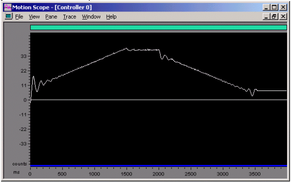
Figure 13. Position Error vs. Time for a Commanded Motion
Kvff = 45, SR = 10,000
PID parameters and Kaff scaled for changed sample rate
Notice that a significant position error in the form of a velocity profile appears with the non-scaled Kvff term.
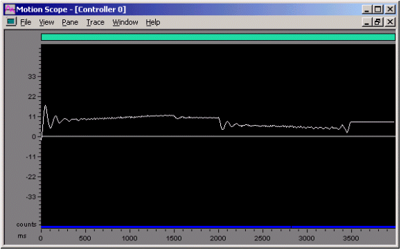
Figure 14. Position Error vs. Time for a Commanded Motion
Kvff = 225, SR =10,000
PID parameters and Kaff scaled for changed sample rate
The position error no longer shows the large velocity profile shaped component. The position error plot is similar in nature to the plot with the original sample rate (SR).
Friction feedforward is not affected by the sample rate, since it has no time component.
Position feedforward is not affected by the sample rate, since it has no time component.
The control system bandwidth cannot exceed the Nyquist Frequency (½ sample rate). This means that there will only be DAC quantization distortions exciting resonances above ½ the sample rate.
This means that if your stage has a large resonance at 3,000 Hz, and you run your controller at a SR = 2,000 Hz, you may never know that the resonance exists. If you change the sample rate to 10,000 Hz, you now have a control system that can create significant 3,000 Hz energy. It would not be surprising to find your stage oscillating at 3,000 Hz.
It is good to know where all the resonances are in your system. If you want to raise your sample rate to a frequency that covers a resonance in your system, consider applying a low pass or notch filter to reduce the magnitude of the resonance.
Do not be afraid of fine tuning the scaled tuning parameters (Hint: write them down first). It is easier to fine tune scaled parameters than to start applying filters. Applying filters will most likely require the use of revised tuning parameters, so it is easier to fine tune scaled parameters instead.
Remember that this method of tuning parameter scaling only provides scaled tuning parameters. It does not take resonances or non-linearities into account, and is not intended to compensate for those effects.
|
Term
|
Compensation
|
| Proportional - Kp | None |
| Integral - Ki | new Ki = old Ki * (old SR / new SR) |
| Derivative - Kd | new Kd = old Kd * (new SR / old SR) |
| Acceleration Feedforward - Kaff | new Kaff = (new SR / old SR)2 * old Kaff |
| Velocity Feedforward - Kvff | new Kvff = (new SR / old SR) * old Kvff |
| Friction Feedforward - Kfff | None |
| Position Feedforward - Kpff | None |
Previous | Back to Table of Contents
| | | Copyright © 2001-2021 Motion Engineering |