|
|
| . |
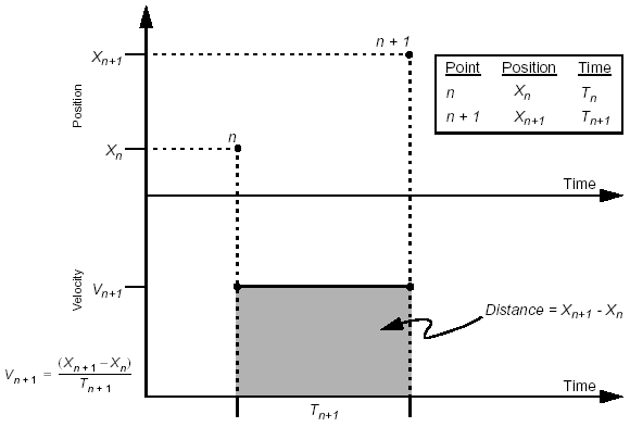
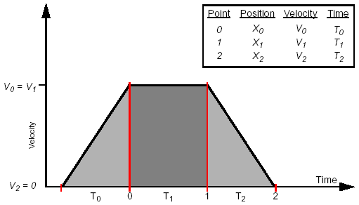
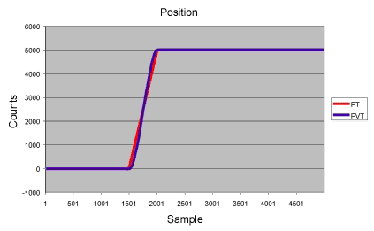
PT and PVT Path MotionIntroductionThis document describes the position-time (PT) and position-velocity-time (PVT) path interpolation algorithms for the XMP controller. A technical description of each algorithm pointing out the advantages and disadvantages is contained in the following sections of this document. General CharacteristicsPT and PVT algorithms convert a series of point-time pairs into XMP motion frames that create the real-time command positions at each sample during the time intervals between the point-time pairs. The PVT interpolation type requires additional data at each point (the vector velocity). A “point” in these point-time series may have several dimensions (axes). PT AlgorithmThe PT algorithm fits a simple constant velocity profile between the user specified “Position and Time” points. The PT algorithm guarantees that the XMP’s trajectory calculator will exactly hit each specified position at the specified time. The constant velocity segment is simply calculated by the difference of the positions divided by the time interval:
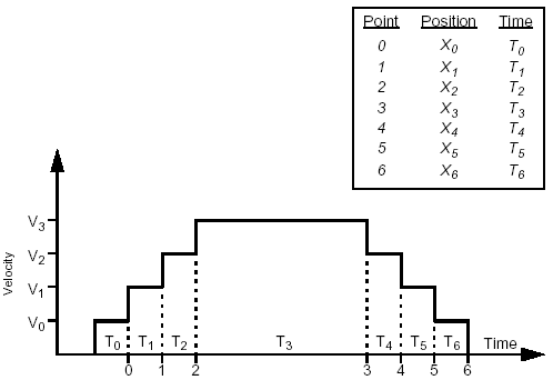
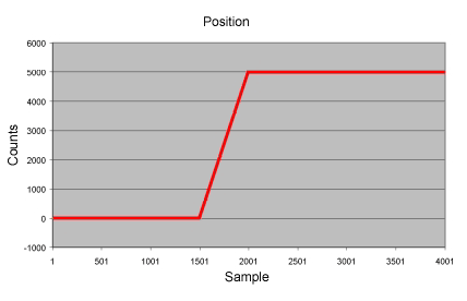
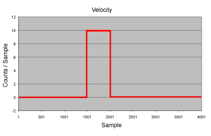
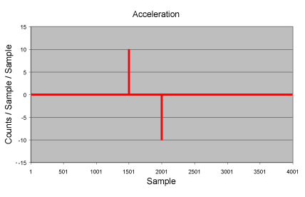
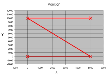
Simple PT ExampleFor example, a trapezoidal velocity profile motion could be generated using a list of Position and Time points:
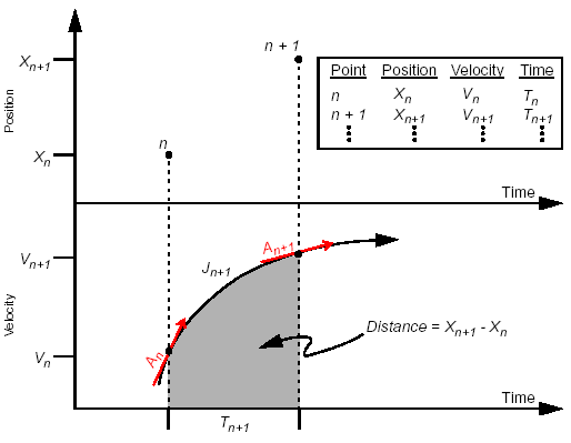
When is the PT algorithm useful?The PT algorithm is very good for closely spaced points or low velocities. It is a very simple algorithm, requiring very few calculations; therefore, it is fast. It works well with low performance motion systems. If the points are spaced too far apart, the motion will be rough, because the acceleration between each point is instantaneous. It is best to keep the point spacing within a few samples. The XMP-Series default sample rate is 500 microseconds. PVT AlgorithmThe PVT algorithm fits a Jerk (non-constant acceleration) profile between user specified "Position, Velocity, and Time" points. The PVT algorithm guarantees that the XMP's trajectory calculator will exactly hit each specified position, with each specified velocity, at the specified time.
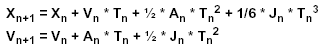
For each point, the PVT algorithm calculates the Acceleration and Jerk values to exactly hit the specified Position and Velocity at the next point. The equations for An and Jn, are derived from the standard kinematic equations:
The derivation of the kinematic equations in terms of An and Jn is beyond the scope of this document. Simple PVT ExampleFor example, a trapezoidal velocity profile motion could be generated using a list of three Position, Velocity, and Time points:
How do you calculate the Velocities for PVT paths? There are several methods to calculate the velocities, depending on the desired path profile. Here are some common methods:
|
||||||||||||||||||||||||||||||||||||||||||||||
Time (samples) |
Position (counts) |
Velocity (PVT only) |
0 |
0 |
0 |
500 |
0 |
0 |
1000 |
0 |
0 |
1500 |
0 |
0 |
2000 |
5000 |
0 |
2500 |
5000 |
0 |
3000 |
5000 |
0 |
3500 |
5000 |
0 |
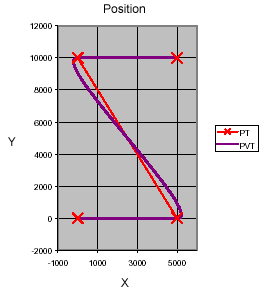
The step is useful for determining if the algorithm is going to have problems in sections of a path with sharp corners. The amount of overshoot (if any), the closeness to lines joining the points, and accelerations and velocities near the step can be evaluated. The step is also useful for determining how much of the path will be affected by a sharp corner (at what distance from the step does the path return to a straight line). For example steps affect Cubic spline interpolation over the entire path, where PT interpolation is only affected at the two points closest to the step.
The zigzag path (really a reversed “Z”) was used to evaluate sharp corner behavior in a two-dimensional (X-Y) path. The following point list formed the zigzag path:
Time (samples) |
X,Y (counts) |
Vx, Vy (counts/sec.,PVT only) |
0 |
0,0 |
0,0 |
500 |
5000,0 |
20000,0 |
1000 |
0,10000 |
20000,0 |
1500 |
5000,1000 |
0,0 |
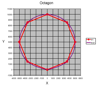
The octagon path determines how well the interpolation algorithms are suited for circular sections of a path. The nine points along the path are on a circle with a radius of 5000 counts, centered at 0,5000. The first and last points are the same (at 0,0 the 6 o’clock position) and the points are spaced at angles of 45 degrees.
This is the simplest form of interpolation. The interpolation is linear (first order). While the path is mathematically continuous, velocity, acceleration, and jerk are not. The lines between points are straight and are traversed at constant speed. PT motion will usually be rough unless the points are very closely spaced in time or the velocities are very low.
PT motion is well suited for paths composed of straight lines and sharp corners. The only serious problem with PT motion is the large number of points required to limit the peak accelerations. In this example the peak acceleration was 40 million c/sec/ sec.
The path is simply straight lines joining the points.
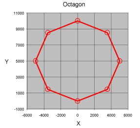
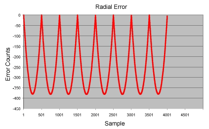
Again, the path consists of simple straight lines. Radial error is the difference between he distance from the interpolated path to the center from the radius of a circle through the points. The largest error is midway between the points.
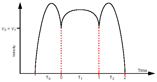
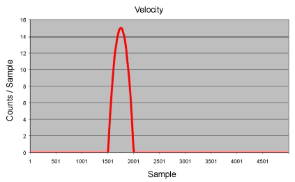
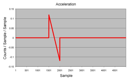
PVT paths are third order (cubic) rather than first order (ex: PT paths). The position and velocity are continuous, the acceleration and jerk are not. PVT paths tend to be much smoother than PT paths, but the velocity of each axis needs to be provided at each of the supplied points. This can increase the complexity of the application since the velocity at each point is often difficult to determine.
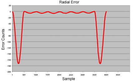
The larger error in the first and last segments is caused by the V=0 constraints at
the end points.
| | | Copyright © 2001-2021 Motion Engineering |