PIV: Tuning the Velocity Loop

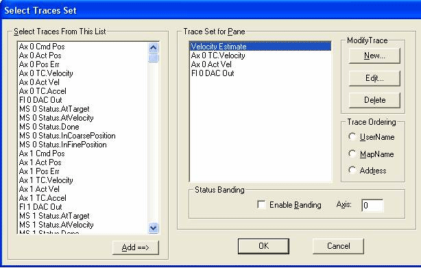
The following tutorial is designed to walk you through the main steps of tuning a system using the PIV algorithm.

Before You Start

When tuning the velocity loop, you will need a way of monitoring velocity loop performance. Fortunately, you can easily accomplish this in Motion Scope by selecting the appropriate traces. Remember, at this point we are not interested in position loop performance. It is worth the effort to set up the traces in a convenient fashion in Motion Scope by clicking the "Traces" button.

In Motion Scope, we will want to look at the following traces:

To learn how to retrieve this data in Motion Scope, please see Monitoring Velocity Loop Performance for detailed instructions.

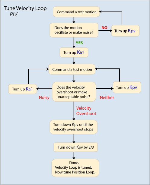
Tuning the Velocity Loop

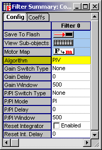
First, we need to make sure that we have the PIV loop enabled (PID is the default). To do this, make sure that Motion Scope Filter Summary Config Algorithm is set to PIV (this sets the algorithm on the controller).

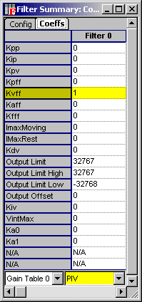
On the Coeffs tab, make sure that the window displays the PIV labels by verifying that the lower right combo box is set to PIV.

Coefficients:
Set all coefficients to 0 with the exception of Kvff
      Kvff = 1
      Kpv = 1            for medium to low resolution systems
      Kpv = 0.01        for high resolution systems or systems with poor mechanics
      Output Limits    these should already be configured.

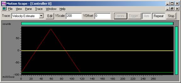
Command a test move. If you see no movement during the move, turn up Kpv x10 or so. In the screenshot below, there is no movement when Kpv = 1.

NOTE: When tuning the velocity loop, Kvff will normally not be adjusted from 1. This is because the PIV loop knows the actual and commanded velocities of the stage. No adjustment is needed in normal systems.

	1,000 count move                           50,000 count / sec velocity             300,000 count / sec2 accel / decel	Red - Commanded Velocity              Green - Actual Velocity                    Yellow - DAC Output (velocity error) White - Velocity Estimate
	Kpv = 1

Since we had no motion, we will increase Kpv to 10.

	1,000 count move                           50,000 count / sec velocity             300,000 count / sec2 accel / decel	Red - Commanded Velocity              Green - Actual Velocity                    Yellow - DAC Output (velocity error) White - Velocity Estimate
	Kpv = 10

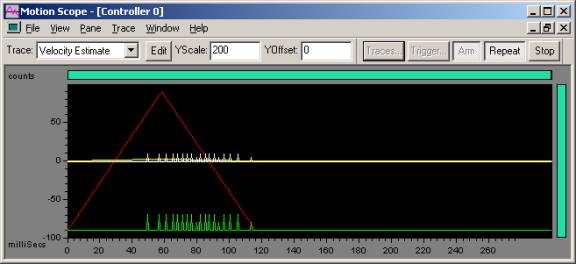
Since we had no motion, we will increase Kpv to 100.

	1,000 count move                           50,000 count / sec velocity             300,000 count / sec2 accel / decel	Red - Commanded Velocity              Green - Actual Velocity                    Yellow - DAC Output (velocity error) White - Velocity Estimate
	Kpv = 100

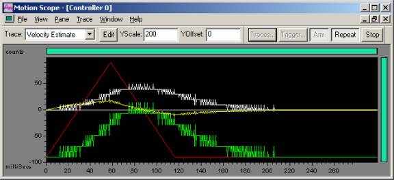
As you can see, there is a hint of motion (the green spikes are encoder counts). Since we can see some motion, we will now double Kpv instead of increasing it x10.

	1,000 count move                           50,000 count / sec velocity             300,000 count / sec2 accel / decel	Red - Commanded Velocity              Green - Actual Velocity                    Yellow - DAC Output (velocity error) White - Velocity Estimate
	Kpv = 200

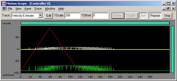
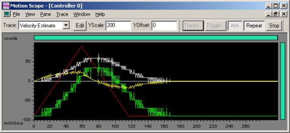
Because we grouped actual velocity (green) and commanded velocity (red) together at the beginning of the program, they are on the same scale. We can see that the actual velocity is nowhere near the commanded velocity and also has a phase delay. It basically means that the actual velocity trace is flattened and is to the right of the commanded velocity trace. The velocity estimate also looks like the actual velocity trace, but scaled differently.

Continue to increase Kpv until the commanded velocity and actual velocity are very similar or until we see instability.

	1,000 count move                           50,000 count / sec velocity             300,000 count / sec2 accel / decel	Red - Commanded Velocity              Green - Actual Velocity                    Yellow - DAC Output (velocity error) White - Velocity Estimate
	Kpv = 500

	1,000 count move                           50,000 count / sec velocity             300,000 count / sec2 accel / decel	Red - Commanded Velocity              Green - Actual Velocity                    Yellow - DAC Output (velocity error) White - Velocity Estimate
	Kpv = 1000

	1,000 count move                           50,000 count / sec velocity             300,000 count / sec2 accel / decel	Red - Commanded Velocity              Green - Actual Velocity                    Yellow - DAC Output (velocity error) White - Velocity Estimate
	Kpv = 2000

	1,000 count move                           50,000 count / sec velocity             300,000 count / sec2 accel / decel	Red - Commanded Velocity              Green - Actual Velocity                    Yellow - DAC Output (velocity error) White - Velocity Estimate
	Kpv = 5000

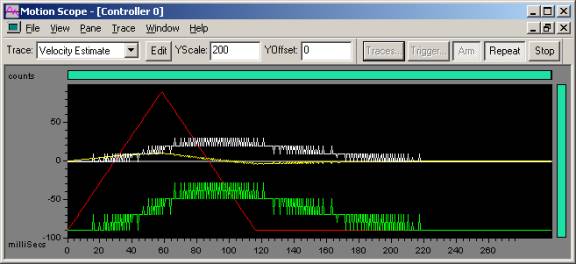
We will stop when Kpv = 5000 because while the motion is stable, it is emitting audible noise that is unacceptable. Notice all the noise on the DAC output. You should also stop turning up Kpv when there is instability (continued position dithering) or an excessive ringing on acceleration transitions.

Also note that as we increased Kpv, the actual velocity profile stretched vertically and shifted to the left as it closed in on the commanded velocity trace.

Why is there such noise on the actual velocity?
Actual velocity on the XMP is measured in encoder counts per sample (2000 Hz = 0.5 msec default sample rate). The commanded move reaches a maximum velocity of about 17,000 counts/sec. This traslates to about 8.5 counts/sample at a 2000 Hz sample rate (default XMP sample rate). Since encoder counts have no fractional part, this means that there are 8 integer values for velocity to 8.5 counts/sample. 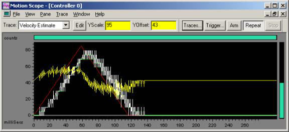When you are traveling at exactly 8.5 counts/sec, you will get 8 counts the first sample, 9 counts the next, 8 the next and so on.

While we are looking at the actual velocity, let's adjust the velocity estimate scaling. The velocity estimate register we are looking at is actually the velocity estimate (counts/sample) * 10. Adjust the Yscale and Yoffset for the velocity estimate until it covers the actual velocity. This will help show the effects of the low pass section we will apply next.

	1,000 count move                           50,000 count / sec velocity             300,000 count / sec2 accel / decel	Red - Commanded Velocity              Green - Actual Velocity                    Yellow - DAC Output (velocity error) White - Velocity Estimate
	Kpv = 5000

Since the only contribution to the DAC output at this point (because the only tuning parameters we have set are Kpv and Kvff) is the velocity error * Kpv, the DAC output is proportional to the velocity error. In other words, the DAC trace at this point is equivalent to the velocity error with different scaling (this is not true if you use tuning parameters other than Kpv and Kvff). If you look at the trace above, you can see that the DAC output is a shape that corresponds to the difference between the actual velocity and the velocity estimate.

Previous | Next